
Printable Excel Formulas Cheat Sheet

An Excel formulas cheat sheet earns its place on your desk when it answers the question you actually have, which is usually "which formula does this job, and how do I write it?" This one covers 37 of the formulas that do most of the work in business spreadsheets, each with its syntax, a plain-English explanation, a worked example, and the mistake people most often make with it.
If you use Excel for work, for a business, or just to keep your life organized, the right formula turns a twenty-minute job into a two-minute one. You do not need to memorize hundreds of functions. You need the right few dozen and a fast way to find them when a task lands in front of you.
Search by formula name or by the task you are trying to finish, tap a category to narrow the list, copy any formula with one click, and print the designed cheat sheet to keep beside your keyboard. Bookmark this page. You will come back to it.
Search the Excel Formulas Cheat Sheet
Search formulasThe Printable Excel Formulas Cheat Sheet
Here is the whole cheat sheet on one designed reference: every formula, its syntax, and what it does, grouped by color, with error codes, reference locking, and shortcuts at the end. Print it in landscape and keep it beside your keyboard. If you have searched or picked a category above, the printout only includes those formulas.
=SUM(A1:A10)=SUM(A1:A10, C1:C10)=AVERAGE(A1:A10)=MIN(A1:A10)=MAX(A1:A10)=COUNT(A1:A10)=COUNTA(A1:A10)=COUNTIF(A1:A10, ">100")=CONCATENATE(A1, " ", B1)=CONCAT(A1, " ", B1)=A1&" "&B1=LEFT(A1, 3)=RIGHT(A1, 4)=MID(A1, 2, 5)=LEN(A1)=TRIM(A1)=UPPER(A1)=LOWER(A1)=PROPER(A1)=SUBSTITUTE(A1, "old text", "new text")=IF(A1>100, "Yes", "No")=AND(A1>100, B1<50)=OR(A1>100, B1<50)=IFS(A1>=90, "A", A1>=80, "B", A1>=70, "C", TRUE, "Below C")=IFERROR(A1/B1, "N/A")=VLOOKUP(A1, B1:D10, 3, FALSE)=HLOOKUP("Mar", B1:M3, 3, FALSE)=INDEX(C1:C10, MATCH(A1, B1:B10, 0))=XLOOKUP(A1, B1:B10, C1:C10)=XLOOKUP(A1, B1:B10, C1:C10, "Not found")=FILTER(A2:D500, C2:C500>500)=FILTER(A2:D500, (C2:C500>500)*(D2:D500="West"), "None")=TODAY()=NOW()=DATEDIF(A1, B1, "D")=DATEDIF(A1, TODAY(), "M")=EDATE(A1, 3)=EOMONTH(A1, 0)=NETWORKDAYS(A1, B1)=NETWORKDAYS(A1, B1, H2:H12)=PMT(rate, nper, pv)=PMT(6%/12, 60, -50000)=NPV(rate, value1, value2, ...)=NPV(8%, B2:B6)-50000=IRR(values)=IRR(B1:B6)=FV(rate, nper, pmt, [pv])=FV(5%/12, 120, -1000)=MEDIAN(A1:A10)=STDEV.S(A1:A10)=STDEV.P(A1:A10)=PERCENTILE.INC(A1:A10, 0.9)=RANK.EQ(A1, $A$1:$A$10, 0)=SUMIF(A1:A10, "North", B1:B10)=SUMIFS(C1:C10, A1:A10, "North", B1:B10, ">100")=AVERAGEIF(A1:A10, "North", B1:B10)=UNIQUE(A1:A10)=TRANSPOSE(A1:A10)Why Excel Formulas Matter
Excel has hundreds of functions, and nobody needs all of them. What you need are the ones that show up in real work every day: totaling revenue, looking up prices, flagging overdue invoices, counting leads, cleaning up imported lists, and working out what a loan will really cost. The formulas on this cheat sheet are those ones, grouped by the job they do.
Knowing the right formula is the difference between spending twenty minutes on a task and spending two. It also cuts errors, because a formula does the same thing every time, while copying numbers by hand eventually slips. Once a sheet is built on formulas, it updates itself when the data changes, and you stop rebuilding the same report every week.
Each formula below gives you the syntax with a copy button, a plain-English explanation of how the formula works, a worked example from a real business task, and the problem people run into most often. In the syntax lines, A1:A10 and similar ranges are placeholders, so swap in the cells from your own sheet after you paste.
Basic Arithmetic Formulas
These are the foundation, and everything else on this cheat sheet builds on them. If you only use Excel to add up columns and count rows, these five formulas will already save you time every week.
SUM
=SUM(A1:A10)=SUM(A1:A10, C1:C10)SUM is the formula most people learn first, and for good reason. It adds every number in the range you give it and quietly skips text and blank cells, so a column with a header or a few empty rows still totals correctly. You can hand it several ranges separated by commas, such as =SUM(B2:B13, D2:D13), when the numbers you need are not side by side.
Say your monthly revenue sits in cells B2 through B13. Typing =SUM(B2:B13) in B14 gives you the total for all twelve months, and if you correct a single month later, the total updates on its own. The same formula totals timesheet hours, expense categories, and units sold, which is why it shows up in almost every business spreadsheet.
The most common SUM problem is numbers stored as text. Figures pasted from a website or exported from another system often land as text, and SUM ignores them without any warning, so the total looks reasonable but comes up short. If a total seems low, check whether the numbers are left-aligned or show a small green triangle, then convert them with Data, Text to Columns. The keyboard shortcut Alt and = writes a SUM for you.
AVERAGE
=AVERAGE(A1:A10)AVERAGE adds up the numbers in a range and divides by how many numbers there are, giving you the arithmetic mean. Like SUM, it ignores text and truly empty cells, but it does count cells that contain a zero, and that difference matters more than most people expect.
If daily sales for the month are in B2:B31, =AVERAGE(B2:B31) tells you what a typical day brings in. Compare that figure against individual days and you quickly see which days pull the month up and which drag it down, which is useful when you are planning staffing or deciding when to run a promotion.
Watch for zeros that really mean "no data yet." If you pre-fill a sheet with 0 for days that have not happened, AVERAGE counts them and understates the result. Leave future cells blank instead, or use =AVERAGEIF(B2:B31, ">0") to average only the days with sales. When one huge value skews the result, MEDIAN, covered further down, gives a truer middle.
MIN and MAX
=MIN(A1:A10)=MAX(A1:A10)MIN returns the lowest number in a range and MAX returns the highest. Both ignore text and blank cells, and both accept several ranges or individual values separated by commas, so =MAX(B2:B50, 0) returns zero if every value in the range is negative.
If you are reviewing a month of customer orders in C2:C200, =MIN(C2:C200) shows your smallest order and =MAX(C2:C200) shows your largest. Subtract one from the other, =MAX(C2:C200)-MIN(C2:C200), and you have the range of your order sizes, a quick sense of how spread out your customers really are.
MAX is also a handy way to put a floor under a calculation. =MAX(0, B2-C2) never returns a negative number, which is exactly what you want for remaining budget or hours left on a contract. MIN does the reverse and caps a value, so =MIN(40, D2) limits regular hours to forty. If you need the smallest or largest value that meets a condition, newer versions of Excel include MINIFS and MAXIFS.
COUNT and COUNTA
=COUNT(A1:A10)=COUNTA(A1:A10)COUNT and COUNTA look alike but answer different questions. COUNT tallies only the cells that contain numbers, including dates, which Excel stores as numbers. COUNTA tallies every cell that is not empty, whether it holds a number, text, a date, or even an error.
Picture a lead list with names in column A and deal values in column C. =COUNTA(A2:A500) tells you how many leads you have in total, and =COUNT(C2:C500) tells you how many of them have a deal value entered. The gap between the two is the number of leads that still need a value, which makes a quick completeness check before a pipeline review.
COUNTA has one trap: it counts cells that look blank but are not, such as a cell holding a single space or a formula that returns an empty string (""). If your count seems too high, that is usually why. COUNTBLANK counts the empty cells, and pairing it with COUNTA is a fast way to audit a column before you rely on it.
COUNTIF
=COUNTIF(A1:A10, ">100")COUNTIF counts only the cells that meet a condition you set. It takes two arguments: the range to look at and the criteria to test. The criteria can be a number, a comparison written in quotes such as ">100", a piece of text such as "Paid", or a reference to another cell.
With order values in C2:C500, =COUNTIF(C2:C500, ">500") tells you exactly how many orders topped $500 without filtering or scrolling. With a status column, =COUNTIF(D2:D500, "Overdue") counts overdue invoices, and the count refreshes every time a status changes.
To compare against a value in another cell, join the operator and the cell with an ampersand: =COUNTIF(C2:C500, ">"&F1). Writing ">F1" inside the quotes does not work, because Excel reads it as the literal text F1. Wildcards help with text, so =COUNTIF(A2:A500, "*Inc*") counts every name containing "Inc." When you need two or more conditions at once, switch to COUNTIFS.
Text Formulas
Text formulas are underrated. If you work with names, addresses, product codes, or any data imported from another system, these formulas clean and reshape text in seconds instead of hours of retyping.
CONCATENATE and CONCAT
=CONCATENATE(A1, " ", B1)=CONCAT(A1, " ", B1)=A1&" "&B1CONCATENATE joins text from several cells, or text you type, into a single string. CONCAT is its newer replacement and does the same job while also accepting whole ranges, so =CONCAT(A2:C2) joins three cells at once. The ampersand operator does the same work with less typing, and many people prefer it: =A2&" "&B2.
With first names in column A and last names in column B, =CONCAT(A2, " ", B2) in column C returns a full name such as "Maria Lopez." Fill it down and every row gets a full name. The same pattern builds product labels, mailing lines, or matching keys such as =A2&"-"&B2 for lining up records across two sheets.
Remember to add the spaces and punctuation yourself, because Excel joins exactly what you give it and nothing else. Numbers also lose their formatting when joined, so $1,250 becomes 1250 unless you wrap it in TEXT, as in =A2&" owes "&TEXT(B2, "$#,##0"). When you need a separator between many cells, TEXTJOIN adds it for you and can skip blanks: =TEXTJOIN(", ", TRUE, A2:E2).
LEFT, RIGHT, and MID
=LEFT(A1, 3)=RIGHT(A1, 4)=MID(A1, 2, 5)LEFT, RIGHT, and MID extract part of a text string. LEFT takes a set number of characters from the start, RIGHT takes them from the end, and MID starts at a position you choose and takes as many characters as you ask for. Together they break apart codes, IDs, and any text that follows a consistent pattern.
Suppose your product codes look like "FUR-10482-BLK." =LEFT(A2, 3) returns "FUR," the category. =RIGHT(A2, 3) returns "BLK," the color. =MID(A2, 5, 5) starts at the fifth character and returns "10482," the item number. Put each in its own column and you can sort, filter, and total by category in seconds.
These formulas always return text, even when the result looks like a number, so "10482" will not add up with SUM or match a numeric lookup. Wrap the result in VALUE to convert it. When the pieces vary in length, combine the formulas with FIND to locate a separator, such as =LEFT(A2, FIND("-", A2)-1), which returns everything before the first dash. Newer versions of Excel also offer TEXTBEFORE and TEXTAFTER for this job.
LEN
=LEN(A1)LEN returns the number of characters in a cell, counting letters, numbers, punctuation, and spaces. On its own it sounds minor, but it is one of the fastest ways to spot data entry problems in a long list.
If every customer ID in your system should be eight characters long, =LEN(A2) in a helper column shows any ID that is too short or too long. Combine it with IF, as in =IF(LEN(A2)<>8, "Check", ""), and you get a flag on every row that needs attention. It works just as well for phone numbers, ZIP codes, and SKU lists.
Because LEN counts spaces, it is also the best way to find hidden ones. If =LEN(A2) returns a bigger number than the characters you can see, the cell has extra spaces at the start or end, which is often why a lookup fails. Run the text through TRIM and compare the two lengths to confirm.
TRIM
=TRIM(A1)TRIM removes leading and trailing spaces from text and shrinks any run of spaces between words down to a single space. It does not change the letters themselves, so it is safe to run across an entire column of imported names or product descriptions.
Contact lists exported from another system often arrive with stray spaces, so " Jane Smith " sits in a cell looking almost normal. =TRIM(A2) returns "Jane Smith." This matters most for lookups, because VLOOKUP and XLOOKUP treat "Jane Smith " and "Jane Smith" as different values, so trimming both sides is often the fix for a lookup that returns #N/A for no obvious reason.
TRIM only removes the standard space character. Data copied from web pages often contains non-breaking spaces, character 160, which TRIM leaves in place. For those, use =TRIM(SUBSTITUTE(A2, CHAR(160), " ")). Once the cleaned column looks right, copy it and use Paste Values over the original so you are not left depending on a helper column.
UPPER, LOWER, and PROPER
=UPPER(A1)=LOWER(A1)=PROPER(A1)These three formulas change the case of text. UPPER converts every letter to capitals, LOWER converts every letter to lowercase, and PROPER capitalizes the first letter of each word and lowercases the rest. None of them change spaces, numbers, or punctuation.
Customer names from an old database often arrive in all caps. =PROPER(A2) turns "JOHN SMITH" into "John Smith" across thousands of rows at once. LOWER is the go-to for email addresses, since =LOWER(B2) makes every address consistent before you remove duplicates, and UPPER keeps state abbreviations and product codes uniform.
PROPER is not perfect with names. It turns "McDonald" into "Mcdonald," and because it capitalizes any letter that follows a non-letter, it turns "it's" into "It'S." Scan the results before anything goes out to customers and fix the few exceptions by hand. As with TRIM, finish by pasting the results as values.
SUBSTITUTE
=SUBSTITUTE(A1, "old text", "new text")SUBSTITUTE swaps one piece of text for another inside a cell. You give it the cell, the text to find, and the text to put in its place. It is case sensitive, and by default it replaces every occurrence, though an optional fourth argument lets you replace only a specific one, such as the second.
If your product names all include "Basic" and you are renaming the tier to "Starter," =SUBSTITUTE(A2, "Basic", "Starter") handles every row at once while leaving the original list untouched for reference. Replacing with nothing removes text entirely, so =SUBSTITUTE(B2, "-", "") strips the dashes out of phone numbers or part numbers.
Nest SUBSTITUTE to make several replacements in one cell. For example, =SUBSTITUTE(SUBSTITUTE(A2, "(", ""), ")", "") removes both parentheses. Because it is case sensitive, "basic" and "Basic" are treated as different words, so clean the case first with LOWER or PROPER if your data is mixed. When you want to replace characters by position instead of by content, use REPLACE.
Logical Formulas
Logical formulas make your spreadsheet think. They are where Excel stops being a calculator and starts making decisions for you, flagging rows, assigning tiers, and hiding errors automatically.
IF
=IF(A1>100, "Yes", "No")IF checks whether a condition is true and returns one result if it is and a different result if it is not. It takes three arguments: the logical test, the value if true, and the value if false. The results can be text in quotes, numbers, cell references, or even other formulas.
With monthly sales in B2, =IF(B2>=10000, "Target Met", "Below Target") labels every row based on performance, and the label changes the moment the number does. IF can calculate as well as label, so =IF(C2>40, (C2-40)*D2*1.5, 0) returns overtime pay only for rows where hours exceed forty.
Nesting more than two or three IFs inside each other gets hard to read and easy to break, so switch to IFS or a lookup table once the rules pile up. Keep text results in quotes and numbers without quotes, since "100" in quotes is text and will not add up. If you leave the last argument out, IF returns FALSE instead of a blank, so use "" when you want the cell to look empty.
AND and OR
=AND(A1>100, B1<50)=OR(A1>100, B1<50)AND returns TRUE only when every condition you give it is true. OR returns TRUE when at least one of them is. On their own they simply show TRUE or FALSE, so most of the time you use them inside IF to turn several checks into one decision.
To flag customers who have placed more than five orders and spent more than $1,000, use =IF(AND(B2>5, C2>1000), "VIP", ""). To flag invoices that need attention because they are either overdue or disputed, use =IF(OR(D2="Overdue", E2="Disputed"), "Follow Up", "").
You can combine the two, such as =AND(B2>5, OR(C2="North", C2="East")), but keep an eye on the parentheses, because one misplaced bracket changes the logic without producing an error. A good habit is to test the AND or OR on its own in a spare column first, confirm the TRUE and FALSE results look right, and only then wrap it in IF.
IFS
=IFS(A1>=90, "A", A1>=80, "B", A1>=70, "C", TRUE, "Below C")IFS tests a list of conditions in order and returns the result paired with the first one that is true. It replaces the stack of IF inside IF inside IF that tiered rules usually need, and it is available in newer versions of Excel, including Microsoft 365.
For a sales tier, =IFS(B2>=50000, "Gold", B2>=25000, "Silver", B2>=10000, "Bronze", TRUE, "None") assigns every rep a tier in one readable formula. The order matters. Excel stops at the first true test, so list the thresholds from highest to lowest, or a big number will land in the wrong tier.
IFS has no built-in "otherwise" value. If none of the conditions are true, it returns #N/A, which is why the example ends with TRUE, "None" as a catch-all. For long tiered lists such as shipping rates or discount levels, a small lookup table with XLOOKUP or VLOOKUP set to an approximate match is easier to maintain than a very long IFS.
IFERROR
=IFERROR(A1/B1, "N/A")IFERROR wraps around another formula. If that formula works, you see its normal result. If it returns any error, such as #N/A, #DIV/0!, or #VALUE!, you see whatever you put in the second argument instead: a message, a zero, or a blank.
Average order value is revenue divided by orders, but in a month with no orders the division throws #DIV/0!. =IFERROR(B2/C2, 0) shows zero instead. The most common use is around lookups, as in =IFERROR(VLOOKUP(A2, Prices!A:C, 3, FALSE), "Not found"), so a missing product shows a clear message rather than an error that breaks the totals below it.
IFERROR hides every error, including the ones that point to a real problem such as a typo in a range. Build and test the formula first, and add IFERROR only once you know it works. When you only want to catch missing lookup values, IFNA is safer because it handles #N/A and lets the other errors show. Our guide to handling and blanking out Excel errors explains what each error means and how to fix it.
Lookup Formulas
Lookup formulas are among the most useful in Excel. They pull information from one table into another automatically, which is the heart of almost every price list, invoice, and report.
VLOOKUP
=VLOOKUP(A1, B1:D10, 3, FALSE)VLOOKUP searches down the first column of a table for a value and returns something from the same row, in a column you specify by number. It takes four arguments: what to look for, the table to search, the column number to return, and whether you want an exact match (FALSE) or an approximate one (TRUE).
With product IDs in column A of your order sheet and a price list on a sheet called Prices, =VLOOKUP(A2, Prices!$A$2:$C$200, 3, FALSE) finds each ID and returns its price from the third column. The dollar signs lock the table in place so it does not shift when you fill the formula down.
Always type FALSE for the last argument unless you truly want an approximate match. Leaving it out makes Excel assume TRUE, which can return the wrong row without any error at all. VLOOKUP also cannot look to the left of the search column, and the column number breaks if someone inserts a column in the table. If you have a newer version of Excel, XLOOKUP avoids all three problems.
HLOOKUP
=HLOOKUP("Mar", B1:M3, 3, FALSE)HLOOKUP is VLOOKUP turned on its side. It searches across the top row of a table for your value and returns the value from the same column, a set number of rows down. The arguments mirror VLOOKUP: what to find, the table, the row number to return, and FALSE for an exact match.
If your budget has months across row 1, with rent in row 2 and payroll in row 3, =HLOOKUP("Mar", B1:M3, 3, FALSE) returns the March payroll figure. Replace "Mar" with a cell reference and you have a report that switches months when you change a single cell.
HLOOKUP carries the same weaknesses as VLOOKUP: it cannot look above its search row, and its row number breaks when rows are inserted. Most people rarely need it, because XLOOKUP searches rows and columns alike. If your data is laid out sideways, it is also worth asking whether flipping it with TRANSPOSE would make the rest of your work easier.
INDEX and MATCH
=INDEX(C1:C10, MATCH(A1, B1:B10, 0))INDEX and MATCH are two formulas that become a powerful lookup when combined. MATCH finds the position of a value in a list, such as the fifth row. INDEX returns whatever sits at a given position in another range. Put MATCH inside INDEX and you can look up a value in one column and return the matching value from any other column.
Suppose your customer sheet has emails in column B and customer IDs in column D, and you need the email for the ID in F2. VLOOKUP cannot look to the left, but =INDEX(B2:B500, MATCH(F2, D2:D500, 0)) can. MATCH finds which row holds the ID, and INDEX returns the email from that same row.
The 0 at the end of MATCH means exact match, and forgetting it is the most common mistake, since the default is an approximate match that expects sorted data. Make sure both ranges start and end on the same rows, or the results will be off by a row. For two-way lookups, add a second MATCH for the column: =INDEX(B2:M50, MATCH(P1, A2:A50, 0), MATCH(P2, B1:M1, 0)).
XLOOKUP
=XLOOKUP(A1, B1:B10, C1:C10)=XLOOKUP(A1, B1:B10, C1:C10, "Not found")XLOOKUP is the modern replacement for VLOOKUP, HLOOKUP, and most INDEX and MATCH combinations. You give it the value to find, the range to search, and the range to return from. It defaults to an exact match, works left or right and up or down, and does not need a column number.
To find a customer's email from their name, =XLOOKUP(F2, B2:B500, C2:C500) searches the names in column B and returns the email from column C. Add a fourth argument, =XLOOKUP(F2, B2:B500, C2:C500, "Not found"), and missing names show a friendly message without wrapping everything in IFERROR. Because the return range is its own argument, inserting a column never breaks it.
The search range and the return range must be the same size, or XLOOKUP returns #VALUE!. It is only available in Microsoft 365 and newer versions of Excel, so people opening your file in an older version will see errors where your lookups should be. Microsoft's XLOOKUP guide covers the optional match mode and search mode arguments if you want to go further.
FILTER
=FILTER(A2:D500, C2:C500>500)=FILTER(A2:D500, (C2:C500>500)*(D2:D500="West"), "None")FILTER returns every row from a range that meets one or more conditions, and it spills the results into as many cells as it needs. Unlike the Filter button on the Data tab, the result is a live formula, so when your source data changes, the filtered list updates on its own.
With a sales table in A2:D500, =FILTER(A2:D500, C2:C500>500) returns every order over $500. To add a second condition, multiply them: =FILTER(A2:D500, (C2:C500>500)*(D2:D500="West"), "None") returns orders over $500 from the West region only and shows "None" when nothing qualifies. Use a plus sign instead of the asterisk when either condition should count.
FILTER needs empty space below and to the right to spill into. If anything is in the way, even a stray space, you get a #SPILL! error until you clear it. Without the third argument, a filter that finds nothing returns #CALC!, so it is worth including a message. FILTER is available in Microsoft 365 and newer versions of Excel.
Date and Time Formulas
Date formulas track deadlines, measure durations, and schedule renewals. Excel stores every date as a number behind the scenes, which is why you can add, subtract, and compare dates like any other value.
TODAY and NOW
=TODAY()=NOW()TODAY returns the current date and NOW returns the current date and time. Neither takes any arguments, and both recalculate every time the workbook recalculates, so the value is current whenever you open the file.
In a project tracker with due dates in column C, =C2-TODAY() returns the number of days left until each deadline, and a negative number means the task is overdue. Pair it with IF, as in =IF(C2<TODAY(), "Overdue", ""), and overdue rows flag themselves every morning without anyone touching the sheet.
Because they always change, TODAY and NOW are the wrong choice for recording when something happened. To stamp a fixed date, press Ctrl and ; to enter today's date as a value, or Ctrl and Shift and ; for the current time. If a subtraction like =C2-TODAY() shows a date instead of a number, change the cell format to General or Number.
DATEDIF
=DATEDIF(A1, B1, "D")=DATEDIF(A1, TODAY(), "M")DATEDIF calculates the difference between two dates in complete days, months, or years. You give it a start date, an end date, and a unit in quotes: "D" for days, "M" for complete months, and "Y" for complete years. Excel keeps it for compatibility and does not list it in the formula suggestions, so you have to type it out in full.
With customer signup dates in column B, =DATEDIF(B2, TODAY(), "M") returns how many full months each customer has been with you, which is useful for loyalty tiers or churn analysis. Use "Y" for employee tenure in whole years, or join "Y" and "YM" to show something like "3 years, 4 months": =DATEDIF(B2, TODAY(), "Y")&" years, "&DATEDIF(B2, TODAY(), "YM")&" months".
The start date must come before the end date, or DATEDIF returns #NUM!. Microsoft also warns that the "MD" unit can return inaccurate results, so avoid it. If you only need days, simply subtracting one date from the other gives the same answer with less typing.
EDATE
=EDATE(A1, 3)EDATE returns the date that falls a given number of months before or after a starting date. Positive numbers move forward and negative numbers move back. It is the right way to add months, because months have different lengths and adding 30 days at a time drifts off course.
For subscriptions that renew twelve months after they start, =EDATE(B2, 12) returns every renewal date from the start dates in column B. For a quarterly check-in, =EDATE(B2, 3) returns the date three months on. Set the result cell to a date format, since EDATE returns the underlying date number.
EDATE handles month ends sensibly. A start date of January 31 plus one month returns the last day of February rather than spilling into March. If you need the last day of the month every time, and not only when the date happens to land there, use EOMONTH instead.
EOMONTH
=EOMONTH(A1, 0)EOMONTH returns the last day of a month, counted a set number of months from a starting date. A zero returns the end of the same month, 1 returns the end of the next month, and -1 returns the end of the previous month.
If invoices are due at the end of the month they are issued, =EOMONTH(B2, 0) returns the due date for every invoice. For terms of end of month plus 30 days, use =EOMONTH(B2, 0)+30. And =EOMONTH(B2, -1)+1 returns the first day of the month, which is handy for grouping transactions in monthly reports.
Like EDATE, EOMONTH returns a date serial number, so format the cell as a date if you see a five-digit number instead. It is also a reliable way to count the days in a month, since =DAY(EOMONTH(B2, 0)) returns 28, 29, 30, or 31 depending on the month.
NETWORKDAYS
=NETWORKDAYS(A1, B1)=NETWORKDAYS(A1, B1, H2:H12)NETWORKDAYS counts the working days between two dates, including both the start and end dates and skipping Saturdays and Sundays. An optional third argument takes a list of holiday dates to skip as well.
A project that starts on a Monday and finishes on the Friday of the following week took 10 working days, and =NETWORKDAYS(B2, C2) returns exactly that. Put your company holidays in a small range such as H2:H12 and use =NETWORKDAYS(B2, C2, $H$2:$H$12) to measure turnaround times, service levels, or time to hire in true business days.
If your team works a different pattern, such as Sunday through Thursday, NETWORKDAYS.INTL lets you choose which days count as the weekend. To go the other direction and find a date a set number of working days ahead, such as a deadline ten business days out, use WORKDAY.
Financial Formulas
Financial formulas are built for business decisions. Loans, savings goals, and investments all come down to money moving over time, and these formulas do that math for you before you commit to anything.
PMT
=PMT(rate, nper, pv)=PMT(6%/12, 60, -50000)PMT calculates the fixed payment needed to pay off a loan over a set number of periods at a constant interest rate. It needs three things: the interest rate per period, the number of periods, and the loan amount, which Excel calls the present value.
Considering a $50,000 equipment loan at 6% annual interest over five years? =PMT(6%/12, 60, -50000) returns about $966.64 a month. The rate is divided by 12 and the term is 60 months because the payments are monthly. Change the rate or the term and you can compare offers before you ever sit down with a lender.
Match the rate and the number of periods to the payment frequency. Using 6% with 60 periods would calculate as if every month charged 6%, and the payment would come out wildly high. Excel also shows money going out as a negative number, so enter the loan amount as a negative, as above, to get a positive payment. PMT covers principal and interest only, not fees or insurance.
NPV
=NPV(rate, value1, value2, ...)=NPV(8%, B2:B6)-50000NPV, or net present value, converts a series of future cash flows into what they are worth today at a discount rate you choose. The discount rate is usually your cost of borrowing or the return you could earn elsewhere. A positive result means the project earns more than that rate, and a negative result means it earns less.
A new product line costs $50,000 up front and is expected to return $15,000 a year for five years. With the five returns in B2:B6 and an 8% discount rate, =NPV(8%, B2:B6)-50000 returns about $9,891. The positive number says the project beats an 8% return, so on these assumptions it is worth pursuing.
The most common NPV mistake is including the up-front cost inside the formula. NPV assumes the first value arrives one period from now, so it discounts everything it is given. Leave the initial investment out and subtract it separately, as in the example. The cash flows also need to be evenly spaced. For irregular dates, use XNPV.
IRR
=IRR(values)=IRR(B1:B6)IRR, or internal rate of return, finds the rate at which a series of cash flows would have a net present value of exactly zero. In plain terms, it tells you the annual return an investment produces, so you can compare it with a loan rate or with other projects.
Using the same project, put the up-front cost as a negative number, -50000, in B1 and the five yearly returns of 15000 in B2:B6. =IRR(B1:B6) returns about 15.2%. If your money costs 8% to borrow, a project returning roughly 15% clears the bar comfortably.
IRR needs at least one negative and one positive value, or it returns #NUM!. Unlike NPV, the up-front cost goes inside the range, as the first value. Like NPV, it assumes evenly spaced periods, so use XIRR when cash flows land on irregular dates. When projects differ a lot in size, look at NPV as well, because a small project can have a high IRR while earning fewer total dollars.
FV
=FV(rate, nper, pmt, [pv])=FV(5%/12, 120, -1000)FV, or future value, calculates what an investment will be worth after a set number of periods, based on a regular payment and a fixed interest rate. You can also include a starting balance as the optional fourth argument.
If you save $1,000 a month at 5% annual interest, =FV(5%/12, 120, -1000) shows the balance after ten years: about $155,282. Of that, $120,000 is money you put in and the rest is interest. Add a starting balance, such as =FV(5%/12, 120, -1000, -10000), to include money you have already saved.
As with PMT, divide an annual rate by 12 and count periods in months when payments are monthly. Deposits are money leaving your pocket, so enter them as negative numbers to get a positive result. FV assumes the rate never changes, so treat the answer as a planning estimate rather than a promise.
Statistical Formulas
Statistical formulas help you understand your data beyond totals and averages: what is typical, how much it varies, and where a single value stands against the rest.
MEDIAN
=MEDIAN(A1:A10)MEDIAN returns the middle value in a set of numbers once they are sorted from smallest to largest. With an even count, it averages the two middle values. Because it looks at position rather than size, a few extremely high or low values barely move it.
Salaries are the classic example. One very high earner can pull the average well above what most people make, while =MEDIAN(C2:C40) returns the true middle. The same logic applies to order values, deal sizes, and days to pay an invoice, where a single huge order or one very late payment would distort an average.
Put AVERAGE and MEDIAN side by side. If they are close, your data is fairly balanced. If the average is much higher than the median, a few large values are pulling it up, and the median is the better number to report as typical. Like AVERAGE, MEDIAN ignores text and blank cells but counts zeros.
STDEV
=STDEV.S(A1:A10)=STDEV.P(A1:A10)Standard deviation measures how far values typically sit from the average. A small number means the values cluster tightly and are consistent, while a large number means they swing widely. STDEV.S is for a sample of data and is the one most people should use. STDEV.P is for when you have every value in the full population. The older STDEV still works and matches STDEV.S.
Suppose seven days of sales are $1,200, $1,350, $980, $1,500, $1,100, $1,420, and $1,250. The average is about $1,257, and =STDEV.S(B2:B8) returns about $182. Most days land within a couple of hundred dollars of the average, which tells you sales are fairly steady and that staffing and inventory can be planned around a stable number.
Standard deviation is easier to judge next to the average. Dividing one by the other, =STDEV.S(B2:B8)/AVERAGE(B2:B8), gives the coefficient of variation, about 14% here, which lets you compare the steadiness of products or locations with very different sales levels.
PERCENTILE
=PERCENTILE.INC(A1:A10, 0.9)PERCENTILE returns the value that a given percentage of your data falls at or below. You give it the range and a percentile written as a decimal between 0 and 1, so 0.9 is the 90th percentile and 0.5 is the median. Newer versions of Excel call it PERCENTILE.INC, and the original PERCENTILE still works the same way.
To find what it takes to be in your top 10% of customers by order value, use =PERCENTILE.INC(C2:C500, 0.9). If ten orders were $75, $85, $95, $120, $180, $260, $340, $410, $510, and $630, the 90th percentile is $522, so any order above that puts a customer in your top tier.
Excel interpolates between values, which is why the result above, $522, is not one of the actual orders. That is normal. For quartiles, QUARTILE.INC is a shortcut. To go the other way and find which percentile a specific value sits at, use PERCENTRANK.INC.
RANK
=RANK.EQ(A1, $A$1:$A$10, 0)RANK returns the position of a number within a list. A 0 or an empty last argument ranks from largest to smallest, so the top value is 1. A 1 ranks from smallest to largest, which is what you want for things like response times, where lower is better. Newer versions call it RANK.EQ, and the older RANK behaves the same way.
With monthly sales per rep in C2:C15, =RANK.EQ(C2, $C$2:$C$15, 0) in column D gives each rep a position, and the leaderboard updates itself whenever the numbers change. Sort by column D, or use conditional formatting to highlight the top three.
Lock the list with dollar signs, as above, or the range shifts as you fill the formula down and the ranks come out wrong. Ties share the same rank and the next rank is skipped, so two reps tied for 2nd are followed by 4th. If you prefer tied values to share an averaged rank, use RANK.AVG.
Conditional and Array Formulas
Conditional and array formulas work across whole ranges at once. They total, average, and reshape data based on rules you set, which makes them the backbone of summary reports.
SUMIF and SUMIFS
=SUMIF(A1:A10, "North", B1:B10)=SUMIFS(C1:C10, A1:A10, "North", B1:B10, ">100")SUMIF adds the values that meet a single condition, and SUMIFS adds values that meet two or more. They are the easiest way to build a summary report: totals by region, by customer, by month, or by any category in your data.
With regions in column A and revenue in column C, =SUMIF(A2:A500, "North", C2:C500) returns total revenue for the North region. To total only large orders from the North, use =SUMIFS(C2:C500, A2:A500, "North", C2:C500, ">500"). Point the criteria at a cell instead of typing "North," and one formula copied down a list of regions builds the entire summary.
Watch the argument order, because the two formulas differ. SUMIF puts the range to add last, while SUMIFS puts it first, followed by pairs of ranges and criteria. Every range must be the same size. For dates, join the operator to a cell, such as ">="&F1, to total everything on or after the date in F1.
AVERAGEIF
=AVERAGEIF(A1:A10, "North", B1:B10)AVERAGEIF averages only the values that meet a condition. The arguments follow SUMIF: the range to test, the criteria, and, optionally, the range to average. If you leave out the third argument, Excel averages the tested range itself.
To find the average order size for orders over $200, use =AVERAGEIF(C2:C500, ">200"). To find the average order size for one sales rep, use =AVERAGEIF(B2:B500, "Dana", C2:C500). Both give you a segment's average without filtering the data or building a separate table.
If no cells meet the condition, AVERAGEIF returns #DIV/0!, because it would be dividing by zero. Wrap it in IFERROR if that can happen in your report. When you need more than one condition, such as one rep in one region, use AVERAGEIFS, which puts the average range first, just as SUMIFS does.
UNIQUE
=UNIQUE(A1:A10)UNIQUE returns a list of the distinct values in a range, each one appearing only once. Like FILTER, it spills the results into the cells below and updates whenever the source changes, so it is a live alternative to the Remove Duplicates button.
If a sales log lists customer names many times over, =UNIQUE(B2:B1000) returns each customer once. Wrap it in COUNTA, =COUNTA(UNIQUE(B2:B1000)), and you know how many distinct customers you have. Combine it with SORT, =SORT(UNIQUE(B2:B1000)), for an alphabetical customer list that grows as new customers appear.
UNIQUE treats "Acme" and "Acme " with a trailing space as two different customers, so clean the column with TRIM first. It needs empty space to spill into, just like FILTER, and it is available in Microsoft 365 and newer versions of Excel. If the source range includes blank cells, the result includes a 0 for them, so size the range to your data.
TRANSPOSE
=TRANSPOSE(A1:A10)TRANSPOSE flips a range on its side, turning rows into columns and columns into rows. In Microsoft 365 and newer versions, it spills the flipped result automatically. In older versions, you select the destination range first and enter the formula with Ctrl and Shift and Enter.
If monthly figures run down column B but your report or chart needs them across a row, =TRANSPOSE(B2:B13) lays the twelve months out side by side. Because it is a formula, the transposed version stays linked to the original, so edits in column B flow straight through.
If you just need a one-time flip and do not want the link, copy the range, then use Paste Special and tick Transpose. That produces plain values you can edit freely. The formula version cannot be partly edited, because typing into any cell of the spilled result breaks it with a #SPILL! error, so choose the version that fits how you will use the data.
The Formulas That Matter Most for Business
If you only learn ten Excel formulas, make them these. Each name links back to its card on this page, so you can jump straight to the syntax and the worked example.
| # | Formula | Why It Matters |
|---|---|---|
| 1 | SUM | Totals revenue, costs, and hours |
| 2 | AVERAGE | Finds typical values, such as average order size |
| 3 | IF | Turns rules into automatic decisions |
| 4 | VLOOKUP or XLOOKUP | Pulls prices, names, and details from other tables |
| 5 | INDEX and MATCH | Flexible lookups that do not break |
| 6 | SUMIF and SUMIFS | Totals by customer, month, or category |
| 7 | COUNTIF | Counts orders, tasks, or leads that meet a rule |
| 8 | IFERROR | Keeps reports clean when data is missing |
| 9 | TRIM | Cleans imported data so lookups work |
| 10 | PMT | Calculates loan and lease payments |
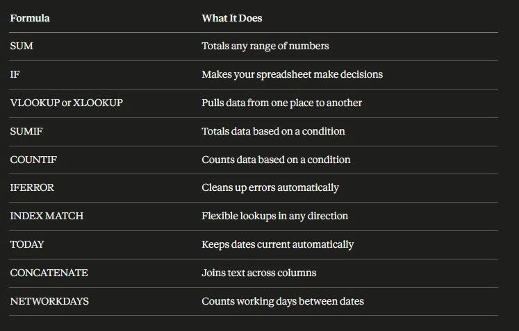
Start with the first four, which cover most everyday spreadsheet tasks, and add the rest as real work calls for them. A formula you learn to solve a problem sitting in front of you sticks far better than one memorized from a list, so the next time a task feels repetitive, search this page for the formula that does it for you.
Keyboard Shortcuts That Speed Up Formula Work
A handful of shortcuts make writing and checking formulas noticeably faster, especially once you are working in larger sheets.
| Shortcut (Windows) | What It Does |
|---|---|
| Alt and = | Inserts a SUM for the cells above or to the left |
| F4 | Cycles a reference between relative and absolute, such as A1 and $A$1 |
| Ctrl and ` | Shows formulas instead of results, so you can check your work |
| Ctrl and D | Copies the formula from the cell above |
| Ctrl and ; | Enters today's date as a fixed value |
| Ctrl and Shift and Enter | Enters a legacy array formula in older versions |
| Ctrl and T | Turns a range into a Table so formulas grow with your data |
On a Mac, most of these use Command in place of Ctrl, and F4 becomes Command and T.
Using These Formulas in Google Sheets
Almost every formula on this cheat sheet works in Google Sheets with the same name and the same arguments. SUM, AVERAGE, IF, IFS, VLOOKUP, INDEX and MATCH, XLOOKUP, SUMIFS, COUNTIF, TEXTJOIN, UNIQUE, the date formulas, and the financial formulas all carry over, so a sheet built in one program usually works in the other without changes.
There are a few differences worth knowing. In Google Sheets, FILTER usually takes each condition as its own argument, as in =FILTER(A2:D500, C2:C500>500, D2:D500="West"), and it has no argument for a no-results message. Sheets also has functions Excel lacks, such as QUERY for SQL-style summaries and IMPORTRANGE for pulling data in from another spreadsheet. Excel, in turn, offers some advanced statistical and financial functions that Google Sheets does not fully support.
Take Your Excel Skills Further
Knowing formulas is the foundation. Knowing how to build real business tools in Excel, such as dashboards, trackers, financial models, and reporting systems, is what takes you from competent to genuinely valuable.
If you want to go deeper, our free Excel courses walk you through everything from the formulas in this guide to building complete business systems from scratch. You will learn how to think in Excel, not just how to copy formulas. Whether you are a small business owner who wants control of your numbers or a professional who wants to move faster with data, the lessons give you a practical, real-world education in Excel that you can apply from day one.
You can also watch the free Excel course videos or keep our guide to 10 Excel functions every user should know handy. For the full list of functions, Microsoft keeps an alphabetical Excel functions reference.
When a whole team depends on spreadsheets for hours, projects, and invoices, Updoot keeps that work in one system as business management software for $5 per user per month, and every tool still exports to Excel.
Opens in Google Drive. View and download for free.
Related Reading
10 Excel Functions Every User Should Know →
Frequently Asked Questions About Excel Formulas
What are the most important Excel formulas to learn first?
Start with SUM, AVERAGE, IF, and VLOOKUP. These four formulas cover the majority of everyday Excel tasks. Once you are comfortable with them, add SUMIF, COUNTIF, IFERROR, and INDEX MATCH to your toolkit and you will be able to handle almost any spreadsheet task you encounter.
What is the difference between VLOOKUP and INDEX MATCH?
VLOOKUP searches left to right only and requires you to specify a column number that can break if columns are inserted or deleted. INDEX MATCH is more flexible, can search in any direction, and does not break when your spreadsheet structure changes. For simple lookups VLOOKUP works fine. For anything complex, INDEX MATCH is the better habit.
What is the difference between VLOOKUP and XLOOKUP?
XLOOKUP is the modern replacement for VLOOKUP. It has simpler syntax, works in any direction, does not require a column number, and handles errors more cleanly. If you are using a recent version of Excel or Microsoft 365, learn XLOOKUP instead of VLOOKUP. Older versions of Excel do not support it.
Do Excel formulas work in Google Sheets?
Most do. SUM, AVERAGE, IF, VLOOKUP, INDEX MATCH, COUNTIF, SUMIF, and most text and date functions work identically in both. The main differences are that Google Sheets has some unique functions like QUERY and IMPORTRANGE that do not exist in Excel, while Excel has some advanced financial and statistical functions that Google Sheets does not fully support.
Why is my Excel formula showing an error?
The most common errors are: a reference to an empty or wrong cell, a division by zero, a VLOOKUP that cannot find the search value, or a mismatch between the data type the formula expects and what is actually in the cell. Wrap your formula in =IFERROR to handle errors gracefully, and double check that your cell references are pointing to the right place.
What is the fastest way to learn Excel formulas?
The fastest way is to learn by doing. Pick a real task you do at work, identify the formula that solves it, and build a spreadsheet around that one formula. Once it clicks in a real context, it sticks. Trying to memorize a formula list in isolation is the slowest approach. Apply each formula to something that actually matters to you and you will retain it immediately.
Can you combine multiple Excel formulas in one cell?
Yes, and this is where Excel becomes genuinely powerful. Nesting formulas inside each other, such as using IF inside SUMIF, or IFERROR around VLOOKUP, lets you build logic that handles complex real-world scenarios in a single cell. Start with simple formulas, get comfortable with each one individually, and then start combining them as your confidence grows.
What is IFERROR used for?
IFERROR wraps around any formula and returns a value you choose if that formula produces an error. Instead of seeing ugly error codes like #N/A or #DIV/0 in your spreadsheet, you see whatever you specify, such as "Not Found" or a blank cell. It is one of the most practical formulas in Excel for building clean, professional looking spreadsheets.