How to Make a Project Progress Google Sheets and Excel Dashboard

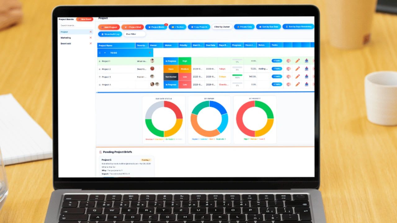
Project progress dashboards in Excel and Google Sheets show at a glance how close each project is to done. Try the free interactive dashboard below, follow the steps to build one with check boxes, color-coded progress bars, and a pie chart, or grab the free templates further down the page.

Here is how the finished dashboard works. Each project has a short list of tasks with check boxes. When a task is checked off, that project's percent complete and progress bar update automatically, and the bar changes from red to yellow to green as the work moves along. At the top, a pie chart combines every project to show overall progress. The same approach works for goals, launches, onboarding checklists, or anything else with steps to complete.

Try the Free Project Progress Dashboard

How to Create a Project Progress Dashboard in Excel

This example tracks four projects with four tasks each, for 16 check boxes in total. The overall progress section sits at the top of the sheet, starting in row 1, and the individual project sections start in row 13.

Set Up the Layout

1. Add and format your main headings. This example uses Overall Project Progress in row 1 and Project Progress in row 13.
2. Add the Project 1 headings starting in row 16, then use the fill color so they stand out. Add borders around the Project 1 section from the Home ribbon. Style it however you like.

Add the Check Boxes

3. Go to the Developer tab, click Insert, choose Check Box, and draw it in place. If you do not see the Developer tab, right-click the ribbon, choose Customize the Ribbon, and check Developer.
4. Copy and paste the check box to create one for each task, then move each into place.
5. Right-click each check box, choose Format Control, and link it to the cell it sits in. Change that cell's font to white so the TRUE or FALSE value is hidden.

Calculate Percent Complete

6. Add a percent-complete formula that divides the checked boxes by the total number of tasks: =COUNTIF(C19:C22,TRUE)/COUNTA(C19:C22)

Build the Progress Bar

7. In the progress bar cell, enter =REPT("|",70*C15) and set the font to Playbill. The formula repeats a thin bar character based on the percent complete, and Playbill turns those characters into a solid bar.

Color the Bar With Conditional Formatting

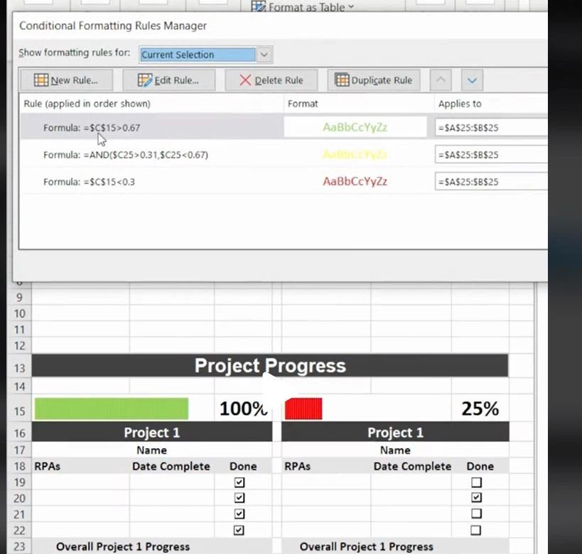
8. Go to Home > Conditional Formatting > New Rule and choose Use a formula to determine which cells to format.
9. For red under 30%, enter =$C$15<0.3 and set the font color to red.
10. Repeat for yellow between 31% and 67% with =AND($C15>0.31,$C15<0.67).
11. Repeat for green above 67% with =$C$15>0.67. Adjust any of these thresholds to fit your projects.

Copy the Section for Each Project

12. Copy the whole Project 1 section and paste it for Projects 2, 3, and 4. Relink each new check box to its own cell.
13. Update the conditional formatting for each copy. Go to Conditional Formatting > Manage Rules and change the cell references to match the new location.
14. Below each project's task list, total the checked boxes, starting in C23: =COUNTIF(C19:C22,TRUE). Adjust the range for each project.

Calculate Overall Progress

15. In row 6, add Completed and Incomplete labels with these formulas:
    Completed: =(C23+C33+G23+G33)/COUNTA(C19:C22,C29:C32,G19:G22,G29:G32)
    Incomplete: =1-F6
16. Spot check your work. With 16 check boxes, check any 8. Completed and Incomplete should both show 50%. If they do not, recheck your ranges.

Add the Pie Chart and Finish the Look

17. Select the Completed and Incomplete labels and percentages, go to Insert, and choose a 3-D pie chart. Click the chart title and delete it.
18. Click each slice and set its fill color. This example uses blue for complete and gray for incomplete.
19. Set the chart background to dark gray. Right-click the chart, choose Format Chart Area, and change the legend text to white under Text Options.
20. Go to View and uncheck Gridlines, then fill the background cells light gray. Your dashboard is done.

How to Create a Project Progress Dashboard in Google Sheets

Google Sheets uses the same layout and the same check box logic, but it builds the progress bar with the SPARKLINE function instead of a font trick.

Set Up the Layout and Progress Bars

1. Add and format your main headings, with Overall Project Progress in row 1 and Project Progress in row 13.
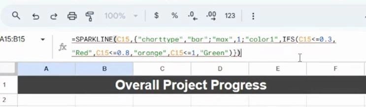
2. Add a progress bar with SPARKLINE. This version shows red up to 30%, orange up to 80%, and green only at 100%. Change the thresholds as you like:
   =SPARKLINE(C15,{"charttype","bar";"max",1;"color1",IFS(C15<=0.3,"Red",C15<=0.8,"Orange",C15<=1,"Green")})

Add the Tasks and Check Boxes

3. Add the Project 1 headings and give them a fill color so they stand out.
4. Select four cells, go to Insert > Checkbox, and the check boxes appear. You can also drag the fill handle down or copy and paste them.
5. Total the checked boxes for the project, starting in C22 (this becomes C23 after you add a row later): =COUNTIF(C19:C22,TRUE)
6. Add borders around the Project 1 section from the toolbar.
7. Add the percent-complete formula and make it large and bold: =COUNTIF(C19:C22,TRUE)/COUNTA(C19:C22)
8. Copy the whole Project 1 section, paste it for Projects 2, 3, and 4, check the formulas, and rename each project.

Calculate Overall Progress and Add the Chart

9. In row 6, add Completed and Incomplete with these formulas:
   Completed: =(C23+C33+G23+G33)/COUNTA(C19:C22,C29:C32,G19:G22,G29:G32)
   Incomplete: =1-F6
10. Select the labels and percentages, go to Insert > Chart, and choose a pie chart. Delete the chart title.
11. Click each slice and set its color, such as blue for complete and gray for incomplete.
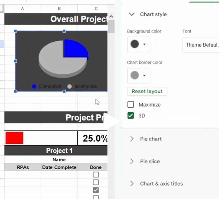
12. Double-click the chart to open the Chart editor. Under Customize > Pie chart, check 3D and try 5% for Distance from center.
13. Color the Completed and Incomplete labels to match the chart, set the chart background to gray, and make the legend text white.

Finish and Test

14. Spot check with 8 of the 16 boxes checked. Completed and Incomplete should both show 50%.
15. Format the Date Complete cells as dates, and add light gray borders to the task cells so they still show once gridlines are off.
16. Go to View > Show and uncheck Gridlines, then fill the background cells light gray. Your dashboard is done.

When a Spreadsheet Dashboard Stops Being Enough

A spreadsheet dashboard is a great way to show progress on a handful of projects. It gets harder to maintain as projects multiply, because every new project means copying sections, relinking check boxes, and updating conditional formatting rules by hand. Updoot project management tracks priority, ownership, status, and progress for every project automatically, with full visibility across teams and no chart to rebuild.